A Blog About the Science and Sociology of Cosmology and Dark Matter
Author: tritonstation
Stacy McGaugh is an astrophysicist and cosmologist who studies galaxies, dark matter, and theories of modified gravity. He is an expert on low surface brightness galaxies, a class of objects in which the stars are spread thin compared to bright galaxies like our own Milky Way. He demonstrated that these dim galaxies appear to be dark matter dominated, providing unique tests of theories of galaxy formation and modified gravity.
Professor McGaugh is currently the chair of the Department of Astronomy at Case Western Reserve University in Cleveland, Ohio, and director of the Warner and Swasey Observatory. Previously he was a member of the faculty at the University of Maryland, having also held research fellowships at Rutgers, the Department of Terrestrial Magnetism of the Carnegie Institution of Washington, and the Institute of Astronomy at the University of Cambridge after earning his Ph.D. from the University of Michigan.
The missing mass problem has been with us many decades now. Going on a century if you start counting from the work of Oort and Zwicky in the 1930s. Not quite a half a century if we date it from the 1970s when most of the relevant scientific community started to take it seriously. Either way, that’s a very long time for a major problem to go unsolved in physics. The quantum revolution that overturned our classical view of physics was lightning fast in comparison – see the discussion of Bohr’s theory in the foundation of quantum mechanics in David Merritt’snew book.
To this day, despite tremendous efforts, we have yet to obtain a confirmed laboratory detection of a viable dark matter particle – or even a hint of persuasive evidence for the physics beyond the Standard Model of Particle Physics (e.g., supersymmetry) that would be required to enable the existence of such particles. We cannot credibly claim (as many of my colleagues insist they can) to know that such invisible mass exists. All we really know is that there is a discrepancy between what we see and what we get: the universe and the galaxies within it cannot be explained by General Relativity and the known stable of Standard Model particles.
If we assume that General Relativity is both correct and sufficient to explain the universe, which seems like a very excellent assumption, then we are indeed obliged to invoke non-baryonic dark matter. The amount of astronomical evidence that points in this direction is overwhelming. That is how we got to where we are today: once we make the obvious, imminently well-motivated assumption, then we are forced along a path in which we become convinced of the reality of the dark matter, not merely as a hypothetical convenience to cosmological calculations, but as an essential part of physical reality.
I think that the assumption that General Relativity is correct is indeed an excellent one. It has repeatedly passed many experimental and observational tests too numerous to elaborate here. However, I have come to doubt the assumption that it suffices to explain the universe. The only data that test it on scales where the missing mass problem arises is the data from which we infer the existence of dark matter. Which we do by assuming that General Relativity holds. The opportunity for circular reasoning is apparent – and frequently indulged.
It should not come as a shock that General Relativity might not be completely sufficient as a theory in all circumstances. This is exactly the motivation for and the working presumption of quantum theories of gravity. That nothing to do with cosmology will be affected along the road to quantum gravity is just another assumption.
I expect that some of my colleagues will struggle to wrap their heads around what I just wrote. I sure did. It was the hardest thing I ever did in science to accept that I might be wrong to be so sure it had to be dark matter – because I was sure it was. As sure of it as any of the folks who remain sure of it now. So imagine my shock when we obtained data that made no sense in terms of dark matter, but had been predicted in advance by a completely different theory, MOND.
When comparing dark matter and MOND, one must weigh all evidence in the balance. Much of the evidence is gratuitously ambiguous, so the conclusion to which one comes depends on how one weighs the more definitive lines of evidence. Some of this points very clearly to MOND, while other evidence prefers non-baryonic dark matter. One of the most important lines of evidence in favor of dark matter is the acoustic power spectrum of the cosmic microwave background (CMB) – the pattern of minute temperature fluctuations in the relic radiation field imprinted on the sky a few hundred thousand years after the Big Bang.
The equations that govern the acoustic power spectrum require General Relativity, but thankfully the small amplitude of the temperature variations permits them to be solved in the limit of linear perturbation theory. So posed, they can be written as a damped and driven oscillator. The power spectrum favors features corresponding to standing waves at the epoch of recombination when the universe transitioned rather abruptly from an opaque plasma to a transparent neutral gas. The edge of a cloud provides an analog: light inside the cloud scatters off the water molecules and doesn’t get very far: the cloud is opaque. Any light that makes it to the edge of the cloud meets no further resistance, and is free to travel to our eyes – which is how we perceive the edge of the cloud. The CMB is the expansion-redshifted edge of the plasma cloud of the early universe.
An easy way to think about a damped and a driven oscillator is a kid being pushed on a swing. The parent pushing the child is a driver of the oscillation. Any resistance – like the child dragging his feet – damps the oscillation. Normal matter (baryons) damps the oscillations – it acts as a net drag force on the photon fluid whose oscillations we observe. If there is nothing going on but General Relativity plus normal baryons, we should see a purely damped pattern of oscillations in which each peak is smaller than the one before it, as seen in the solid line here:
The CMB acoustic power spectrum predicted by General Relativity with no cold dark matter (line) and as observed by the Planck satellite (data points).
As one can see, the case of no Cold Dark Matter (CDM) does well to explain the amplitudes of the first two peaks. Indeed, it was the only hypothesis to successfully predict this aspect of the data in advance of its observation. The small amplitude of the second peak came as a great surprise from the perspective of LCDM. However, without CDM, there is only baryonic damping. Each peak should have a progressively lower amplitude. This is not observed. Instead, the third peak is almost the same amplitude as the second, and clearly higher than expected in the pure damping scenario of no-CDM.
CDM provides a net driving force in the oscillation equations. It acts like the parent pushing the kid. Even though the kid drags his feet, the parent keeps pushing, and the amplitude of the oscillation is maintained. For the third peak at any rate. The baryons are an intransigent child and keep dragging their feet; eventually they win and the power spectrum damps away on progressively finer angular scales (large 𝓁 in the plot).
As I wrote in this review, the excess amplitude of the third peak over the no-CDM prediction is the best evidence to my mind in favor of the existence of non-baryonic CDM. Indeed, this observation is routinely cited by many cosmologists to absolutely require dark matter. It is argued that the observed power spectrum is impossible without it. The corollary is that any problem the dark matter picture encounters is a mere puzzle. It cannot be an anomaly because the CMB tells us that CDM has to exist.
Impossible is a high standard. I hope the reader can see the flaw in this line of reasoning. It is the same as above. In order to compute the oscillation power spectrum, we have assumed General Relativity. While not replacing it, the persistent predictive successes of a theory like MOND implies the existence of a more general theory. We do not know that such a theory cannot explain the CMB until we develop said theory and work out its predictions.
That said, it is a tall order. One needs a theory that provides a significant driving term without a large amount of excess invisible mass. Something has to push the swing in a universe full of stuff that only drags its feet. That does seem nigh on impossible. Or so I thought until I heard a talk by Pedro Ferreira where he showed how the scalar field in TeVeS – the relativistic MONDian theory proposed by Bekenstein – might play the same role as CDM. However, he and his collaborators soon showed that the desired effect was indeed impossible, at least in TeVeS: one could not simultaneously fit the third peak and the data preceding the first. This was nevertheless an important theoretical development, as it showed how it was possible, at least in principle, to affect the peak ratios without massive amounts of non-baryonic CDM.
At this juncture, there are two options. One is to seek a theory that might work, and develop it to the point where it can be tested. This is a lot of hard work that is bound to lead one down many blind alleys without promise of ultimate success. The much easier option is to assume that it cannot be done. This is the option adopted by most cosmologists, who have spent the last 15 years arguing that the CMB power spectrum requires the existence of CDM. Some even seem to consider it to be a detection thereof, in which case we might wonder why we bother with all those expensive underground experiments to detect the stuff.
Rather fewer people have invested in the approach that requires hard work. There are a few brave souls who have tried it; these include Constantinos Skordis and Tom Złosnik. Very recently, the have shown a version of a relativistic MOND theory (which they call RelMOND) that does fit the CMB power spectrum. Here is the plot from their paper:
Note that black line in their plot is the fit of the LCDM model to the Planck power spectrum data. Their theory does the same thing, so it necessarily fits the data as well. Indeed, a good fit appears to follow for a range of parameters. This is important, because it implies that little or no fine-tuning is needed: this is just what happens. That is arguably better than the case for LCDM, in which the fit is very fine-tuned. Indeed, that was a large point of making the measurement, as it requires a very specific set of parameters in order to work. It also leads to tensions with independent measurements of the Hubble constant, the baryon density, and the amplitude of the matter power spectrum at low redshift.
As with any good science result, this one raises a host of questions. It will take time to explore these. But this in itself is a momentous result. Irrespective if RelMOND is the right theory or, like TeVeS, just a step on a longer path, it shows that the impossible is in fact possible. The argument that I have heard repeated by cosmologists ad nauseam like a rosary prayer, that dark matter is the only conceivable way to explain the CMB power spectrum, is simply WRONG.
A Philosophical Approach to MOND is a new book by David Merritt. This is a major development in the both the science of cosmology and astrophysics, on the one hand, and the philosophy and history of science on the other. It should be required reading for anyone interested in any of these topics.
For many years, David Merritt was a professor of astrophysics who specialized in gravitational dynamics, leading a number of breakthroughs in the effects of supermassive black holes in galaxies on the orbits of stars around them. He has since transitioned to the philosophy of science. This may not sound like a great leap, but it is: these are different scholarly fields, each with their own traditions, culture, and required background education. Changing fields like this is a bit like switching boats mid-stream: even a strong swimmer may flounder in the attempt given the many boulders academic disciplines traditionally place in the stream of knowledge to mark their territory. Merritt has managed the feat with remarkable grace, devouring the background reading and coming up to speed in a different discipline to the point of a lucid fluency.
For the most part, practicing scientists have little interaction with philosophers and historians of science. Worse, we tend to have little patience for them. The baseline presumption of many physical scientists is that we know what we’re doing; there is nothing the philosophers can teach us. In the daily practice of what Kuhn called normal science, this is close to true. When instead we are faced with potential paradigm shifts, the philosophy of science is critical, and the absence of training in it on the part of many scientists becomes glaring.
In my experience, most scientists seem to have heard of Popper and Kuhn. If that. Physical scientists will almost always pay lip service to Popper’s ideal of falsifiablity, and that’s pretty much the extent of it. Living up to applying that ideal is another matter. If an idea that is near and dear to their hearts and careers is under threat, the knee-jerk response is more commonly “let’s not get carried away!”
There is more to the philosophy of science than that. The philosophers of science have invested lots of effort in considering both how science works in practice (e.g., Kuhn) and how it should work (Popper, Lakatos, …) The practice and the ideal of science are not always the same thing.
The debate about dark matter and MOND hinges on the philosophy of science in a profound way. I do not think it is possible to make real progress out of our current intellectual morass without a deep examination of what science is and what it should be.
Merritt takes us through the methodology of scientific research programs, spelling out what we’ve learned from past experience (the history of science) and from careful consideration of how science should work (its philosophical basis). For example, all scientists agree that it is important for a scientific theory to have predictive power. But we are disturbingly fuzzy on what that means. I frequently hear my colleagues say things like “my theory predicts that” in reference to some observation, when in fact no such prediction was made in advance. What they usually mean is that it fits well with the theory. This is sometimes true – they could have predicted the observation in advance if they had considered that particular case. But sometimes it is retroactive fitting more than prediction – consistency, perhaps, but it could have gone a number of other ways equally well. Worse, it is sometimes a post facto assertion that is simply false: not only was the prediction not made in advance, but the observation was genuinely surprising at the time it was made. Only in retrospect is it “correctly” “predicted.”
The philosophers have considered these situations. One thing I appreciate is Merritt’s review of the various takes philosophers have on what counts as a prediction. I wish I had known these things when I wrote the recent review in which I took a very restrictive definition to avoid the foible above. The philosophers provide better definitions, of which more than one can be usefully applicable. I’m not going to go through them here: you should read Merritt’s book, and those of the philosophers he cites.
From this philosophical basis, Merritt makes a systematic, dare I say, scientific, analysis of the basic tenets of MOND and MONDian theories, and how they fare with regard to their predictions and observational tests. Along the way, he also considers the same material in the light of the dark matter paradigm. Of comparable import to confirmed predictions are surprising observations: if a new theory predicts that the sun will rise in the morning, that isn’t either new or surprising. If instead a theory expects one thing but another is observed, that is surprising, and it counts against that theory even if it can be adjusted to accommodate the new fact. I have seen this happen over and over with dark matter: surprising observations (e.g., the absence of cusps in dark matter halos, the small numbers of dwarf galaxies, downsizing in which big galaxies appear to form earliest) are at first ignored, doubted, debated, then partially explained with some mental gymnastics until it is Known and of course, we knew it all along. Merritt explicitly points out examples of this creeping determinism, in which scientists come to believe they predicted something they merely rationalized post-facto (hence the preeminence of genuinely a priori predictions that can’t be fudged).
Merritt’s book is also replete with examples of scientists failing to take alternatives seriously. This is natural: we have invested an enormous amount of time developing physical science to the point we have now reached; there is an enormous amount of background material that cannot simply be ignored or discarded. All too often, we are confronted with crackpot ideas that do exactly this. This makes us reluctant to consider ideas that sound crazy on first blush, and most of us will rightly display considerable irritation when asked to do so. For reasons both valid and not, MOND skirts this bondary. I certainly didn’t take it seriously myself, nor really considered it at all, until its predictions came true in my own data. It was so far below my radar that at first I did not even recognize that this is what had happened. But I did know I was surprised; what I was seeing did not make sense in terms of dark matter. So, from this perspective, I can see why other scientists are quick to dismiss it. I did so myself, initially. I was wrong to do so, and so are they.
A common failure mode is to ignore MOND entirely: despite dozens of confirmed predictions, it simply remains off the radar for many scientists. They seem never to have given it a chance, so they simply don’t pay attention when it gets something right. This is pure ignorance, which is not a strong foundation from which to render a scientific judgement.
Another common reaction is to acknowledge then dismiss. Merritt provides many examples where eminent scientists do exactly this with a construction like: “MOND correctly predicted X but…” where X is a single item, as if this is the only thing that [they are aware that] it does. Put this way, it is easy to dismiss – a common refrain I hear is “MOND fits rotation curves but nothing else.” This is a long-debunked falsehood that is asserted and repeated until it achieves the status of common knowledge within the echo chamber of scientists who refuse to think outside the dark matter box.
This is where the philosophy of science is crucial to finding our way forward. Merritt’s book illuminates how this is done. If you are reading these words, you owe it to yourself to read his book.
The distance scale is fundamental to cosmology. How big is the universe? is pretty much the first question we ask when we look at the Big Picture.
The primary yardstick we use to describe the scale of the universe is Hubble’s constant: the H0 in
v = H0 D
that relates the recession velocity (redshift) of a galaxy to its distance. More generally, this is the current expansion rate of the universe. Pick up any book on cosmology and you will find a lengthy disquisition on the importance of this fundamental parameter that encapsulates the size, age, critical density, and potential fate of the cosmos. It is the first of the Big Two numbers in cosmology that expresses the still-amazing fact that the entire universe is expanding.
Quantifying the distance scale is hard. Throughout my career, I have avoided working on it. There are quite enough, er, personalities on the case already.
No need for me to add to the madness.
Not that I couldn’t. The Tully-Fisher relation has long been used as a distance indicator. It played an important role in breaking the stranglehold that H0 = 50 km/s/Mpc had on the minds of cosmologists, including myself. Tully & Fisher (1977) found that it was approximately 80 km/s/Mpc. Their method continues to provide strong constraints to this day: Kourkchi et al. find H0 = 76.0 ± 1.1(stat) ± 2.3(sys) km s-1 Mpc-1. So I’ve been happy to stay out of it.
Until now.
I am motivated in part by the calibration opportunity provided by gas rich galaxies, in part by the fact that tension in independent approaches to constrain the Hubble constant only seems to be getting worse, and in part by a recent conference experience. (Remember when we traveled?) Less than a year ago, I was at a cosmology conference in which I heard an all-too-typical talk that asserted that the Planck H0 = 67.4 ± 0.5 km/s/Mpc had to be correct and everybody who got something different was a stupid-head. I’ve seen this movie before. It is the same community (often the very same people) who once insisted that H0 had to be 50, dammit. They’re every bit as overconfident as before, suffering just as much from confirmation bias (LCDM! LCDM! LCDM!), and seem every bit as likely to be correct this time around.
So, is it true? We have the data, we’ve just refrained from using it in this particular way because other people were on the case. Let’s check.
The big hassle here is not measuring H0 so much as quantifying the uncertainties. That’s the part that’s really hard. So all credit goes to Jim Schombert, who rolled up his proverbial sleeves and did all the hard work. Federico Lelli and I mostly just played the mother-of-all-jerks referees (I’ve had plenty of role models) by asking about every annoying detail. To make a very long story short, none of the items under our control matter at a level we care about, each making < 1 km/s/Mpc difference to the final answer.
In principle, the Baryonic Tully-Fisher relation (BTFR) helps over the usual luminosity-based version by including the gas, which extends application of the relation to lower mass galaxies that can be quite gas rich. Ignoring this component results in a mess that can only be avoided by restricting attention to bright galaxies. But including it introduces an extra parameter. One has to adopt a stellar mass-to-light ratio to put the stars and the gas on the same footing. I always figured that would make things worse – and for a long time, it did. That is no longer the case. So long as we treat the calibration sample that defines the BTFR and the sample used to measure the Hubble constant self-consistently, plausible choices for the mass-to-light ratio return the same answer for H0. It’s all relative – the calibration changes with different choices, but the application to more distant galaxies changes in the same way. Same for the treatment of molecular gas and metallicity. It all comes out in the wash. Our relative distance scale is very precise. Putting an absolute number on it simply requires a lot of calibrating galaxies with accurate, independently measured distances.
Here is the absolute calibration of the BTFR that we obtain:
The Baryonic Tully-Fisher relation calibrated with 50 galaxies with direct distance determinations from either the Tip of the Red Giant Branch method (23) or Cepheids (27).
In constructing this calibrated BTFR, we have relied on distance measurements made or compiled by the Extragalactic Distance Database, which represents the cumulative efforts of Tully and many others to map out the local universe in great detail. We have also benefited from the work of Ponomareva et al, which provides new calibrator galaxies not already in our SPARC sample. Critically, they also measure the flat velocity from rotation curves, which is a huge improvement in accuracy over the more readily available linewidths commonly employed in Tully-Fisher work, but is expensive to obtain so remains the primary observational limitation on this procedure.
Still, we’re in pretty good shape. We now have 50 galaxies with well measured distances as well as the necessary ingredients to construct the BTFR: extended, resolved rotation curves, HI fluxes to measure the gas mass, and Spitzer near-IR data to estimate the stellar mass. This is a huge sample for which to have all of these data simultaneously. Measuring distances to individual galaxies remains challenging and time-consuming hard work that has been done by others. We are not about to second-guess their results, but we can note that they are sensible and remarkably consistent.
There are two primary methods by which the distances we use have been measured. One is Cepheids – the same type of variable stars that Hubble used to measure the distance to spiral nebulae to demonstrate their extragalactic nature. The other is the tip of the red giant branch (TRGB) method, which takes advantage of the brightest red giants having nearly the same luminosity. The sample is split nearly 50/50: there are 27 galaxies with a Cepheid distance measurement, and 23 with the TRGB. The two methods (different colored points in the figure) give the same calibration, within the errors, as do the two samples (circles vs. diamonds). There have been plenty of mistakes in the distance scale historically, so this consistency is important. There are many places where things could go wrong: differences between ourselves and Ponomareva, differences between Cepheids and the TRGB as distance indicators, mistakes in the application of either method to individual galaxies… so many opportunities to go wrong, and yet everything is consistent.
Having followed the distance scale problem my entire career, I cannot express how deeply impressive it is that all these different measurements paint a consistent picture. This is a credit to a large community of astronomers who have worked diligently on this problem for what seems like aeons. There is a temptation to dismiss distance scale work as having been wrong in the past, so it can be again. Of course that is true, but it is also true that matters have improved considerably. Forty years ago, it was not surprising when a distance indicator turned out to be wrong, and distances changed by a factor of two. That stopped twenty years ago, thanks in large part to the Hubble Space Telescope, a key goal of which had been to nail down the distance scale. That mission seems largely to have been accomplished, with small differences persisting only at the level that one expects from experimental error. One cannot, for example, make a change to the Cepheid calibration without creating a tension with the TRGB data, or vice-versa: both have to change in concert by the same amount in the same direction. That is unlikely to the point of wishful thinking.
Having nailed down the absolute calibration of the BTFR for galaxies with well-measured distances, we can apply it to other galaxies for which we know the redshift but not the distance. There are nearly 100 suitable galaxies available in the SPARC database. Consistency between them and the calibrator galaxies requires
H0 = 75.1 +/- 2.3 (stat) +/- 1.5 (sys) km/s/Mpc.
This is consistent with the result for the standard luminosity-linewidth version of the Tully-Fisher relation reported by Kourkchi et al. Note also that our statistical (random/experimental) error is larger, but our systematic error is smaller. That’s because we have a much smaller number of galaxies. The method is, in principle, more precise (mostly because rotation curves are more accurate than linewidhts), so there is still a lot to be gained by collecting more data.
Our measurement is also consistent with many other “local” measurements of the distance scale,
but not with “global” measurements. See the nice discussion by Telescoper and the paper from which it comes. A Hubble constant in the 70s is the answer that we’ve consistently gotten for the past 20 years by a wide variety of distinct methods, including direct measurements that are not dependent on lower rungs of the distance ladder, like gravitational lensing and megamasers. These are repeatable experiments. In contrast, as I’ve pointed out before, it is the “global” CMB-fitted value of the Hubble parameter that has steadily diverged from the concordance region that originally established LCDM.
So, where does this leave us? In the past, it was easy to dismiss a tension of this sort as due to some systematic error, because that happened all the time – in the 20th century. That’s not so true anymore. It looks to me like the tension is real.
Galaxies are big. Our own Milky Way contains about fifty billion solar masses of stars, and another ten billion of interstellar gas, roughly speaking. The average star is maybe half a solar mass, so crudely speaking, that’s one hundred billion stars. Give or take. For comparison, the population of the Earth has not quite reached eight billion humans. So if you gave each one of us our own personal starship, in order to visit every star in the Galaxy, each one of us would have to visit a dozen stars. Give or take. I’m getting old, so I call dibs on Proxima Centauri through Procyon.
Figure 1 shows a picture of NGC 628, a relatively nearby spiral galaxy. What you see here is mostly stars, along with some interstellar dust and ionized gas. In addition to those components, there are also stellar remnants left behind by dead stars (mostly white dwarfs, some neutron stars, and the occasional black hole). In the space between the stars resides colder forms of interstellar gas, including both atomic gas (individual atoms in space) and molecular gas (the cold, dense material from which new stars form). How much is there of each component?
Fig 1. The spiral galaxy NGC 628. The continuum light of stars in contrasted by dark dust lanes and highlighted by pink pinpoints of Balmer line emission. These are regions of interstellar gas illuminated by the UV emission of short-lived, massive O stars. Not visible here is the interstellar atomic and molecular gas from which stars form.
The bulk of the normal mass (excluding dark matter) in big spiral galaxies like the Milky Way is stars and their remnants. But there is also diffuse material in the vast interstellar medium – the ample space between the stars. This includes dust and several distinct phases of gas – molecular, atomic, and ionized (plasma). The dust and plasma are easy to see, but don’t add up to much – a mere millions of solar masses each for the whole Milky Way. The atomic and molecular gas add up to a lot more, but cannot be seen optically.
Atomic gas can be traced by 21 cm emission from the spin-flip transition of atomic hydrogen using radio telescopes. This is commonly referred to with the spectroscopic notation “HI”. The HI mass – the mass of atomic hydrogen – is usually the second largest mass component in spirals, after stars. In dwarf galaxies, the atomic gas often outweighs the stars (Fig. 2).
Fig 2. Gas mass vs. stellar mass for galaxies in the SPARC database (blue) and an independent sample selected from SDSS (grey) by Bradford. The line is the line of equality where gas mass and stellar mass are equal. The red point is the Milky Way. Like other bright spirals, it is more stars than gas. Among lower mass dwarf galaxies, the reverse is commonly true: those in the field have more gas than stars.
Stars and atomic (HI) gas are the big two. When it comes to star forming galaxies, more massive spirals are usually star dominated while less massive dwarfs are usually dominated by atomic gas. But what about molecular gas?
Molecular gas is important to the star formation process. It is the densest (a very relative term!) material in the interstellar medium, the place where cold gas can condense into the nuggets that sometimes form stars. How much of this necessary ingredient is there?
The bulk of the mass of molecular gas is in molecular hydrogen, H2. Spectroscopically, H2 is a really boring molecule. It has no transitions in wavelength regimes that are readily accessible to observation. So, unlike atomic hydrogen, which brazenly announces its presence throughout the universe via the 21 cm line, molecular hydrogen is nigh-on invisible.
So we use proxies. The most commonly employed proxy for tracing molecular gas mass is carbon monoxide. CO is one of many molecules that accompany the much more abundance molecular hydrogen, and CO produces emission features that are more readily accessible observationally in the mm wavelength range. That has made it the tracer of choice.
CO is far from an ideal tracer of mass. Carbon and oxygen are both trace elements compared to hydrogen, so the correspondence between CO emission and molecular gas mass depends on the relative abundance of both. If that sounds dodgy, it gets worse. It also depends on the interstellar radiation field, the opacity thereto (molecular gas is inevitably associated with dense clumps of dust that shield it from the ambient radiation), and the spatial overlap of the two components – CO and H2 thrive in similar but not identical regions of space. Hence, converting the observed intensity of CO into a molecular hydrogen mass is a highly sensitive procedure that we typically bypass by assuming it is a universal constant.
It’s astronomy. We do what we can.
People have obsessed long and hard about the CO-to-H2 conversion, so we do have a reasonable idea what it is. While many debates can be had over the details, we have a decent idea of what the molecular gas mass is in some galaxies, at least to a first approximation. Molecular gas is usually outweighed by atomic gas, but sometimes it is comparable. So we’d like to keep track of it for the mass budget.
Fig 3. The mass in molecular hydrogen gas as a function of atomic hydrogen (left) and stellar mass (right) from xGASS. The dotted line is the line of equality; molecular gas is usually outweighed by both atomic gas and stars. The red line at right is where the molecular gas mass is 7% of the stellar mass.
Obtaining CO observations is expensive, and often impossible: there are a lot of star forming galaxies where it simply isn’t detected. So we presume there is molecular gas there – that’s where the stars form, but we can’t always see it. So it would be handy to have another proxy besides CO.
Atomic gas is a lousy proxy for molecular gas. The mass of one hardly correlates with the other (Fig. 3). The two phases coexist in a complex and ever-changing variable quasi-equilibrium, with the amount of each at any given moment subject to change so that a snapshot of many galaxies provides a big mess.
Fortunately, the molecular gas mass correlates better with other properties – notably star formation. This makes sense, because stars form from molecular gas. So in some appropriately averaged sense, one follows the other. Star formation can be traced in a variety of ways, like the Balmer emission in Fig. 1. We can see the stars forming and infer the amount of molecular gas required to fuel that star formation even if we can’t detect the gas directly (Fig. 4).
Fig 4. The current star formation rate (left) and molecular gas mass (right) as a function of stellar mass. The grey and black points are from xGASS, with the black points being those where the current star formation rate is within a factor of two of the past average (i.e., the stellar mass divided by the age of the universe). Blue points are low surface brightness galaxies. These extend the relation at left to much lower mass, but are generally not detected in CO. The molecular gas at right (open squares) is inferred by the amount required to sustain the observed star formation.
I’ve done a lot of work on low surface brightness galaxies, a class of objects that have proven particularly difficult to detect in CO. They have low dust contents, low oxygen abundances, relatively hard interstellar radiation fields – all factors that mitigate against CO. Yet we do see them forming stars, sometimes just one O star at a time, and we know how much molecular gas it takes to do that. So we can use star formation as a proxy for molecular gas mass. This is probably no worse than using CO, and perhaps even better – or would be, if we didn’t have to rely on CO to calibrate it in the first place.
Accurate tracers of star formation are also somewhat expensive to obtain. There are situations in which we need an estimate for the molecular gas mass where we don’t have either CO or a measurement of the star formation rate. So… we need a proxy for the proxy. Fortunately, that is provided by the stellar mass.
The stellar mass of a star-forming galaxy correlates with both its molecular gas mass and its star formation rate (Figs. 3 and 4). This is not surprising. It takes molecules to form stars, and it takes star formation to build up stellar mass. Indeed, the stellar mass is the time-integral of the star formation rate, so a correlation between the two (as seen in the left panel of Fig. 4) is mathematically guaranteed.
This brings us to the seven percent solution. Going through all the calibration steps, the molecular gas mass is, on average, about 7% of the stellar mass (the red lines in Figs. 3 and 4). The uncertainties in this are considerable. I’ve tried to work this out previously, and typically came up with numbers in the 5 – 10% range. So it seems to be in there somewhere.
This is adequate for some purposes, but not for others. One thing I want it for is to keep track of the total mass budget of baryons in galaxies so that we can calibrate the Baryonic Tully-Fisher relation. For this purpose it is adequate since molecular gas ranks behind both stars and atomic gas in the mass budget of almost every rotating galaxy. If it is 5% or 10% instead of 7%, this is a difference of a few percent of something that is itself typically < 10% of the total, and often less. A few percent of a few percent is a good working definition of negligible – especially in astronomy.
On top of all that, we also have to keep track of the stuff that isn’t hydrogen – helium and everything else in the periodic table, which astronomers often refer to collectively as “metals.” This makes for all sorts of partially-deserved jokes – oxygen isn’t a metal! but it is number 3 in cosmic abundance after hydrogen and helium. Like many anachronisms, the practice has good historical precedent. Early efforts to measure the abundances of the chemical elements in stars first gave results for iron. As other elements were probed, their abundances followed a pattern that scaled pretty well with the abundance of iron relative to hydrogen. So once again we have a proxy – this time, the iron abundance being a stand-in for that of everything else. Hence the persistence of the terminology – the metallicity of a star is a shorthand for the fraction of its mass that is not hydrogen and helium.
And that fraction is small. We usually write the mass fractions of hydrogen, helium, and everything else (metals) as
X + Y + Z = 1
where X is the fraction of mass in hydrogen, Y that in helium, and Z is everything else. For the sun, Lodders gives X = 0.7389, Y = 0.2463, and Z = 0.0148. Do I believe all those significant digits? No. Is there a good reason for them to be there? Yes. So without delving into those details, let’s just note that the universe is about 3 parts hydrogen, one part helium, with a sprinkling of everything else. Everything else being all the elements in the periodic table that aren’t hydrogen or helium – all the carbon and nitrogen and oxygen and silicon and magnesium and noble gases and actual metals – these all add up to about 1.5% of the mass of the sun, which is typical of nearby stars. So you can see why they’re all just metals to many astronomers.
For the mass of gas in galaxies, we need to correct what we measure in hydrogen for the presence of helium and metals. We measure the mass of atomic hydrogen using the 21 cm line, but that’s just the hydrogen. There is a corresponding amount of helium and metals that goes along with it. So we estimate the mass fraction in hydrogen, X, and use divide by that to get the total mass: Mgas = MHI/X. We do the same for molecular gas, etc.
There are measurements of the metallicities of entire galaxies, but – you guessed it – this isn’t observationally cheap, and isn’t always available. So we need another proxy. Luckily for us, it turns out that once again there is a pretty good correlation of metallicity with stellar mass: galaxies with lots of stars have made lots of supernovae that have processed lots of material into metals. Most of it is still hydrogen, so this is a very subtle effect: 1/X = 1.34 for the tiniest dwarf, going up to about 1.4 for a galaxy like the Milky Way. Still, we know this happens, so we can account for it, at least in a statistical way.
For those who are curious about the details, or want the actual formulae to use, please refer to this AAS research note. Next time, I hope to discuss an application for all this.
This is a wise truth that has often been poorly interpreted. I despise some of the results that this sports quote has had in American culture. It has fostered a culture of bad sportsmanship in some places: an acceptance, even a dictum, that the ends justify the means – up to and including cheating, provided you can get away with it.
Winning every time is an impossible standard. In any competitive event, someone will win a particular game, and someone else will lose. Every participant will be on the losing side some of the time. Learning to lose gracefully despite a great effort is an essential aspect of sportsmanship that must be taught and learned, because it sure as hell isn’t part of human nature.
But there is wisdom here. The quote originates with a football coach. Football is a sport where there is a lot of everything – to even have a chance of winning, you have to do everything right. Not just performance on the field, but strategic choices made before and during the game, and mundane but essential elements like getting the right personnel on the field for each play. What? We’re punting? I thought it was third down!
You can do everything right and still lose. And that’s what I interpret the quote to really mean. You have to do everything to compete. But people will only judge you to be successful if you win.
To give a recent example, the Kansas City Chiefs won this year’s Superbowl. It was only a few months ago, though it seems much longer in pandemic time. The Chiefs dominated the Superbowl, but they nearly didn’t make it past the AFC Championship game.
The Tennessee Titans dominated the early part of the AFC Championship game. They had done everything right. They had peaked at the right time as a team in the overly long and brutal NFL season. They had an excellent game plan, just as they had had in handily defeating the highly favored New England Patriots on the way to the Championship game. Their defense admirably contained the high octane Chiefs offense. It looked like they were going to the Superbowl.
Then one key injury occurred. The Titans lost the only defender who could match up one on one with tight end Travis Kelce. This had an immediate impact on the game, as they Chiefs quickly realized they could successfully throw to Kelce over and over after not having been able to do so at all. The Titans were obliged to double-cover, which opened up other opportunities. The Chief’s offense went from impotent to unstoppable.
I remember this small detail because Kelce is a local boy. He attended the same high school as my daughters, playing on the same field they would (only shortly later) march on with the marching band during half times. If it weren’t for this happenstance of local interest, I probably wouldn’t have noticed this detail of the game, much less remember it.
The bigger point is that the Titans did everything right as a team. They lost anyway. All most people will remember is that the Chiefs won the Superbowl, not that the Titans almost made it there. Hence the quote:
“Winning isn’t everything. It’s the only thing.”
The hallmark of science is predictive power. This is what distinguishes it from other forms of knowledge. The gold standard is a prediction that is made and published in advance of the experiment that tests it. This eliminates the ability to hedge: either we get it right in advance, or we don’t.
The importance of such a prediction depends on how surprising it is. Predicting that the sun will rise tomorrow is not exactly a bold prediction, is it? If instead we have a new idea that changes how we think about how the world works, and makes a prediction that is distinct from current wisdom, then that’s very important. Judging how important a particular prediction may be is inevitably subjective.
It is rare that we actually meet the gold standard of a priori prediction, but it does happen. A prominent example is the prediction of gravitational lensing by General Relativity. Einstein pointed out that his theory predicted twice the light-bending that Newtonian theory did. Eddington organized an expedition to measure this effect during a solar eclipse, and claimed to confirm Einstein’s prediction within a few years of it having been made. This is reputed to have had a strong impact that led to widespread acceptance of the new theory. Some of that was undoubtedly due to Eddington’s cheerleading: it does not suffice merely to make a successful prediction, that it has happened needs to become widely known.
It is impossible to anticipate every conceivable experimental result and publish a prediction for it in advance. So there is another situation: does a theory predict what is observed? This has several standards. The highest standard deserves a silver medal. This happens when you work out the prediction of a theory, and you find that it gives exactly what is observed, with very little leeway. If you had had the opportunity to make the prediction in advance, it would have risen to the gold standard.
Einstein provides another example of a silver-standard prediction. A long standing problem in planetary dynamics was the excess precession of the perihelion of Mercury. The orientation of the elliptical orbit of Mercury changes slowly, with the major axis of the ellipse pivoting by 574 arcseconds per century. That’s a tiny rate of angular change, but we’ve been keeping very accurate records of where the planets are for a very long time, so it was well measured. Indeed, it was recognized early that precession would be cause by torques from other planets: it isn’t just Mercury going around the sun; the rest of the solar system matters too. Planetary torques are responsible for most of the effect, but not all. By 1859, Urbain Le Verrier had worked out that the torques from known planets should only amount to 532 arcseconds per century. [I am grossly oversimplifying some fascinating history. Go read up on it!] The point is that there was an excess, unexplained precession of 43 arcseconds per century. This discrepancy was known, known to be serious, and had no satisfactory explanation for many decades before Einstein came on the scene. No way he could go back in time and make a prediction before he was born! But when he worked out the implications of his new theory for this problem, the right answer fell straight out. It explained an ancient and terrible problem without any sort of fiddling: it had to be so.
The data for the precession of the perihelion of Mercury were far superior to the first gravitational lensing measurements made by Eddington and his colleagues. The precession was long known and accurately measured, the post facto prediction clean and irresolute. So in this case, the silver standard was perhaps better than the gold standard. Hence the question once posed to me by a philosopher of science: why we should care if the prediction came in advance of the observation? If X is a consequence of a theory, and X is observed, what difference does it make which came first?
In principle, none. In practice, it depends. I made the hedge above of “very little leeway.” If there is zero leeway, then silver is just as good as gold. There is no leeway to fudge it, so the order doesn’t matter.
It is rare that there is no leeway to fudge it. Theorists love to explore arcane facets of their ideas. They are exceedingly clever at finding ways to “explain” observations that their theory did not predict, even those that seem impossible for their theory to explain. So the standard by which such a post-facto “prediction” must be judged depends on the flexibility of the theory, and the extent to which one indulges said flexibility. If it is simply a matter of fitting for some small number of unknown parameters that are perhaps unknowable in advance, then I would award that a bronze medal. If instead one must strain to twist the theory to make it work out, then that merits at best an asterisk: “we fit* it!” can quickly become “*we’re fudging it!” That’s why truly a priori prediction is the gold standard. There is no way to go back in time and fudge it.
An important corollary is that if a theory gets its predictions right in advance, then we are obliged to acknowledge the efficacy of that theory. The success of a priori predictions is the strongest possible sign that the successful theory is a step in the right direction. This is how we try to maintain objectivity in science: it is how we know when to suck it up and say “OK, my favorite theory got this wrong, but this other theory I don’t like got its prediction exactly right. I need to re-think this.” This ethos has been part of science for as long as I can remember, and a good deal longer than that. I have heard some argue that this is somehow outdated and that we should give up this ethos. This is stupid. If we give up the principle of objectivity, science would quickly degenerate into a numerological form of religion: my theory is always right! and I can bend the numbers to make it seem so.
Hence the hallmark of science is predictive power. Can a theory be applied to predict real phenomena? It doesn’t matter whether the prediction is made in advance or not – with the giant caveat that “predictions” not be massaged to fit the facts. There is always a temptation to massage one’s favorite theory – and obfuscate the extent to which one is doing so. Consequently, truly a priori prediction must necessarily remain the gold standard in science. The power to make such predictions is fundamental.
Predictive power in science isn’t everything. It’s the only thing.
As I was writing this, I received email to the effect that these issues are also being discussed elsewhere, by Jim Baggot and Sabine Hossenfelder. I have not yet read what they have to say.
I haven’t written much here of late. This is mostly because I have been busy, but also because I have been actively refraining from venting about some of the sillier things being said in the scientific literature. I went into science to get away from the human proclivity for what is nowadays called “fake news,” but we scientists are human too, and are not immune from the same self-deception one sees so frequently exercised in other venues.
So let’s talk about something positive. Current grad student Pengfei Li recently published a paper on the halo mass function. What is that and why should we care?
One of the fundamental predictions of the current cosmological paradigm, ΛCDM, is that dark matter clumps into halos. Cosmological parameters are known with sufficient precision that we have a very good idea of how many of these halos there ought to be. Their number per unit volume as a function of mass (so many big halos, so many more small halos) is called the halo mass function.
An important test of the paradigm is thus to measure the halo mass function. Does the predicted number match the observed number? This is hard to do, since dark matter halos are invisible! So how do we go about it?
Galaxies are thought to form within dark matter halos. Indeed, that’s kinda the whole point of the ΛCDM galaxy formation paradigm. So by counting galaxies, we should be able to count dark matter halos. Counting galaxies was an obvious task long before we thought there was dark matter, so this should be straightforward: all one needs is the measured galaxy luminosity function – the number density of galaxies as a function of how bright they are, or equivalently, how many stars they are made of (their stellar mass). Unfortunately, this goes tragically wrong.
Fig. 5 from the review by Bullock & Boylan-Kolchin. The number density of objects is shown as a function of their mass. Colored points are galaxies. The solid line is the predicted number of dark matter halos. The dotted line is what one would expect for galaxies if all the normal matter associated with each dark matter halo turned into stars.
This figure shows a comparison of the observed stellar mass function of galaxies and the predicted halo mass function. It is from a recent review, but it illustrates a problem that goes back as long as I can remember. We extragalactic astronomers spent all of the ’90s obsessing over this problem. [I briefly thought that I had solved this problem, but I was wrong.] The observed luminosity function is nearly flat while the predicted halo mass function is steep. Consequently, there should be lots and lots of faint galaxies for every bright one, but instead there are relatively few. This discrepancy becomes progressively more severe to lower masses, with the predicted number of halos being off by a factor of many thousands for the faintest galaxies. The problem is most severe in the Local Group, where the faintest dwarf galaxies are known. Locally it is called the missing satellite problem, but this is just a special case of a more general problem that pervades the entire universe.
Indeed, the small number of low mass objects is just one part of the problem. There are also too few galaxies at large masses. Even where the observed and predicted numbers come closest, around the scale of the Milky Way, they still miss by a large factor (this being a log-log plot, even small offsets are substantial). If we had assigned “explain the observed galaxy luminosity function” as a homework problem and the students had returned as an answer a line that had the wrong shape at both ends and at no point intersected the data, we would flunk them. This is, in effect, what theorists have been doing for the past thirty years. Rather than entertain the obvious interpretation that the theory is wrong, they offer more elaborate interpretations.
Faced with the choice between changing one’s mind and proving that there is no need to do so, almost everybody gets busy on the proof.
J. K. Galbraith
Theorists persist because this is what CDM predicts, with or without Λ, and we need cold dark matter for independent reasons. If we are unwilling to contemplate that ΛCDM might be wrong, then we are obliged to pound the square peg into the round hole, and bend the halo mass function into the observed luminosity function. This transformation is believed to take place as a result of a variety of complex feedback effects, all of which are real and few of which are likely to have the physical effects that are required to solve this problem. That’s way beyond the scope of this post; all we need to know here is that this is the “physics” behind the transformation that leads to what is currently called Abundance Matching.
Abundance matching boils down to drawing horizontal lines in the above figure, thus matching galaxies with dark matter halos with equal number density (abundance). So, just reading off the graph, a galaxy of stellar mass M* = 108 M☉ resides in a dark matter halo of 1011 M☉, one like the Milky Way with M* = 5 x 10¹⁰ M☉ resides in a 1012 M☉ halo, and a giant galaxy with M* = 1012 M☉ is the “central” galaxy of a cluster of galaxies with a halo mass of several 1014 M☉. And so on. In effect, we abandon the obvious and long-held assumption that the mass in stars should be simply proportional to that in dark matter, and replace it with a rolling fudge factor that maps what we see to what we predict. The rolling fudge factor that follows from abundance matching is called the stellar mass–halo mass relation. Many of the discussions of feedback effects in the literature amount to a post hoc justification for this multiplication of forms of feedback.
This is a lengthy but insufficient introduction to a complicated subject. We wanted to get away from this, and test the halo mass function more directly. We do so by use of the velocity function rather than the stellar mass function.
The velocity function is the number density of galaxies as a function of how fast they rotate. It is less widely used than the luminosity function, because there is less data: one needs to measure the rotation speed, which is harder to obtain than the luminosity. Nevertheless, it has been done, as with this measurement from the HIPASS survey:
The number density of galaxies as a function of their rotation speed (Zwaan et al. 2010). The bottom panel shows the raw number of galaxies observed; the top panel shows the velocity function after correcting for the volume over which galaxies can be detected. Faint, slow rotators cannot be seen as far away as bright, fast rotators, so the latter are always over-represented in galaxy catalogs.
The idea here is that the flat rotation speed is the hallmark of a dark matter halo, providing a dynamical constraint on its mass. This should make for a cleaner measurement of the halo mass function. This turns out to be true, but it isn’t as clean as we’d like.
Those of you who are paying attention will note that the velocity function Martin Zwaan measured has the same basic morphology as the stellar mass function: approximately flat at low masses, with a steep cut off at high masses. This looks no more like the halo mass function than the galaxy luminosity function did. So how does this help?
To measure the velocity function, one has to use some readily obtained measure of the rotation speed like the line-width of the 21cm line. This, in itself, is not a very good measurement of the halo mass. So what Pengfei did was to fit dark matter halo models to galaxies of the SPARC sample for which we have good rotation curves. Thanks to the work of Federico Lelli, we also have an empirical relation between line-width and the flat rotation velocity. Together, these provide a connection between the line-width and halo mass:
The relation Pengfei found between halo mass (M200) and line-width (W) for the NFW (ΛCDM standard) halo model fit to rotation curves from the SPARC galaxy sample.
Once we have the mass-line width relation, we can assign a halo mass to every galaxy in the HIPASS survey and recompute the distribution function. But now we have not the velocity function, but the halo mass function. We’ve skipped the conversion of light to stellar mass to total mass and used the dynamics to skip straight to the halo mass function:
The halo mass function. The points are the data; these are well fit by a Schechter function (black line; this is commonly used for the galaxy luminosity function). The red line is the prediction of ΛCDM for dark matter halos.
The observed mass function agrees with the predicted one! Test successful! Well, mostly. Let’s think through the various aspects here.
First, the normalization is about right. It does not have the offset seen in the first figure. As it should not – we’ve gone straight to the halo mass in this exercise, and not used the luminosity as an intermediary proxy. So that is a genuine success. It didn’t have to work out this well, and would not do so in a very different cosmology (like SCDM).
Second, it breaks down at high mass. The data shows the usual Schechter cut-off at high mass, while the predicted number of dark matter halos continues as an unabated power law. This might be OK if high mass dark matter halos contain little neutral hydrogen. If this is the case, they will be invisible to HIPASS, the 21cm survey on which this is based. One expects this, to a certain extent: the most massive galaxies tend to be gas-poor ellipticals. That helps, but only by shifting the turn-down to slightly higher mass. It is still there, so the discrepancy is not entirely cured. At some point, we’re talking about large dark matter halos that are groups or even rich clusters of galaxies, not individual galaxies. Still, those have HI in them, so it is not like they’re invisible. Worse, examining detailed simulations that include feedback effects, there do seem to be more predicted high-mass halos that should have been detected than actually are. This is a potential missing gas-rich galaxy problem at the high mass end where galaxies are easy to detect. However, the simulations currently available to us do not provide the information we need to clearly make this determination. They don’t look right, so far as we can tell, but it isn’t clear enough to make a definitive statement.
Finally, the faint-end slope is about right. That’s amazing. The problem we’ve struggled with for decades is that the observed slope is too flat. Here a steep slope just falls out. It agrees with the ΛCDM down to the lowest mass bin. If there is a missing satellite-type problem here, it is at lower masses than we probe.
That sounds great, and it is. But before we get too excited, I hope you noticed that the velocity function from the same survey is flat like the luminosity function. So why is the halo mass function steep?
When we fit rotation curves, we impose various priors. That’s statistics talk for a way of keeping parameters within reasonable bounds. For example, we have a pretty good idea of what the mass-to-light ratio of a stellar population should be. We can therefore impose as a prior that the fit return something within the bounds of reason.
One of the priors we imposed on the rotation curve fits was that they be consistent with the stellar mass-halo mass relation. Abundance matching is now part and parcel of ΛCDM, so it made sense to apply it as a prior. The total mass of a dark matter halo is an entirely notional quantity; rotation curves (and other tracers) pretty much never extend far enough to measure this. So abundance matching is great for imposing sense on a parameter that is otherwise ill-constrained. In this case, it means that what is driving the slope of the halo mass function is a prior that builds-in the right slope. That’s not wrong, but neither is it an independent test. So while the observationally constrained halo mass function is consistent with the predictions of ΛCDM; we have not corroborated the prediction with independent data. What we really need at low mass is some way to constrain the total mass of small galaxies out to much larger radii that currently available. That will keep us busy for some time to come.
I was contacted today by a colleague at NASA’s Goddard Space Flight Center who was seeking to return some photographic plates of Halley’s comet that had been obtained with the Burrell Schmidt telescope. I at first misread the email – I get so many requests for data, I initially assumed that he was looking for said plates. That sent me into a frenzy of where the heck are they? about data obtained by others well before my time as the director of the Warner & Swasey Observatory. Comet Halley last came by in 1986.
Fortunately, reading comprehension kicked in, and I realized that all I really needed to figure out was where they should go. The lower pressure version of where the heck are they? That would be the Pisgah Astronomical Research Institute, which has had the good sense to archive the vast treasury of astronomical plates that many observatories obtained in the pre-digital era but don’t always have the ability to preserve. But this post isn’t about that; it is just a spark to the memory.
In 1986, I was a first-year graduate student in the Princeton physics department. As such, I had at that time little more competence in observing the sky than any other physicist (practically none). Nevertheless, I traipsed out into an open field at the dark edge of town on a clear night with a pair of binoculars and a vague knowledge of what part of the sky Comet Halley should be in. How hard could it be to spot the most famous comet in history?
Impossibly hard. There was nothing to see, so far as I could find. The apparition of 1986 was a bust. This informed in me a bad attitude towards comets. There had never been a good apparition in my lifetime (all of 22 years at that point), and Halley certainly wasn’t one. I accepted that decent comets must be a rare occurrence.
Flash forward a decade to 1996, by which time I was an accomplished observer with a good working knowledge of the celestial sphere. A new comet was discovered – Hyakutake – and with it came much hype. Yeah, yeah, I’d heard it all before. Boring. Comets were always a flop.
Comet Hyakutake made a close approach to Earth in March of 1996. Its wikipedia page is pretty good, with a nice illustration of its orbit and its path on the sky as perceived from the Earth. I was working at DTM at the time, where there were lots of planetary scientists as well as a few astronomers. Someone posted an ephemeris, so despite my distrust of comets I found myself peeking at what its trajectory would be. Nevertheless, we had a long period of cloudy weather, so there was nothing to see even if there was something to see, which I expected there wasn’t.
At this time, my elder daughter Caitlyn was two years old. I made a habit of taking her out and pointing things out in the sky. We watched the sunset, the moon set after it near new moon, and the moon rise near full moon. She seemed content to listen to her old man babble about the lights in the sky. Apparently more of that sank in than I realized.
My wife Anne was teaching at Loyola, and her department chair had invited us over for a party around the vernal equinox. We enjoyed the adult company and Caitlyn put up well with it – up to a point. It got dark and we bid our farewells and headed out. We had parked across the street, and on the way out Betsy (our hostess) said “Stacy – you’re an astronomer. Where’s the comet?”
I got this pained expression. Stupid comets. But it had cleared up for the first time in nearly a week, and looking up from the front door, I could quickly orient myself on the sky. Doing so, I realize that the comet was behind the house. So I pointed up and over, towards the back yard and through the roof: “Over there.” I continued across the street to the car with the toddler cradled in my left arm, fiddling with the keys with my right hand.
We did not have a nice car: one had to insert the key manually into the door to unlock it. As I went around the car to get to the driver’s side, I was focused on this mundane task. It did not occur to me to look up in the direction I had just pointed. I felt Caitlyn stretch her arm to point at the sky, exclaiming “Fuzzy thing!”
I looked up. There is was: a big, bright, fuzzy ball. A brilliant cometary apparition, the coma easily visible even in Baltimore. My two-year old daughter spotted it and accurately classified it before I even looked up.
Comet Hyakutake was an amazing event. Not only spectacular to look at, but it drove home celestial mechanics in a visceral way. It was at this time very close to Earth (by the scale of such things). That meant it made noticeable progress in its orbit from night to night. You couldn’t see it moving just staring at it, but one night is was here, the next night it was there, the following night over there. It was skipping through the constellations at a dizzying speed for an object that takes c. 70,000 years to complete one orbit. But we were close enough that one could easily see the progress it made across the sky from night to night, if not minute to minute. If you wanted to take a picture with a telescope, you had to track the telescope to account for this – hence the star trails in the image above: the stars appear as streaks because the telescope is moving with the comet, not with the sky.
The path of Comet Huyakutake across the sky.
This figure (credit: Tom Ruen) shows the orbital path of Comet Huyakutake projected on the sky (constellations outlined in blue). Most of the time, the comet is far away near the aphelion of its orbit. As it fell in towards the sun, its path made annual ellipses due to the reflex motion of the Earth’s own orbit – the parallax. These grew in size until the comet came sweeping by in the month of March, 1996. Think about it: it spent tens of thousands of years spiraling down towards us, only to shoot by, transitioning well across the sky in only a couple of weeks. Celestial mechanics made visible.
Not long after Hyakutake started to fade, Comet Hale-Bopp became visible. Hale-Bopp did not pass as close to the Earth as Hyakutake, so it didn’t leap across the sky like Tom Bombadil. But Hale-Bopp was a physically larger comet. As such, it got bright and stayed bright for a long time, remaining visible to the naked eye for a record year and half. In the months after Hyakutake’s apparition, we could see Hale-Bopp chasing the sunset from the balcony of our apartment. Caitlyn and I would sit there and watch it as the twilight faded into dark. Her experience of comets had been the opposite of mine: where in my thirty years (before that point) they had been rare and disappointing, in her (by then) three years they had been common and spectacular.
The sky is full of marvels. You never know when you might get to see one.
I happened to visit this blog as a visitor from a computer not mine. Seeing it that way made me realize how obnoxious the ads had become. So WordPress’s extortion worked; I’ve agreed to send them a few $ every month to get rid of the ads. With it comes a new domain name: tritonstation.com. Bookmarks to the previous website (tritonstation.wordpress.com) should redirect here. Let me know if a problem arises, or the barrage of ads fails to let up. I may restructure the web page so there is more here than just this blog, but that will have to await my attention in my copious spare time.
As it happens, I depart soon to attend an IAU meeting on galaxy dynamics. This is being held in part to honor the career of Prof. Jerry Sellwood, with whom I had the pleasure to work while a postdoc at Rutgers. He hosted a similar meeting at Rutgers in 1998; I’m sure that some of the same issues discussed then will be debated again next week.
Physics and Astronomy are two fields divided by a common interest in how the universe works. There is a considerable amount of overlap between some sub-fields of these subjects, and practically none at all in others. The aims and goals are often in common, but the methods, assumptions, history, and culture are quite distinct. This leads to considerable confusion, as with the English language – scientists with different backgrounds sometimes use the same words to mean rather different things.
A few terms that are commonly used to describe scientists who work on the subjects that I do include astronomer, astrophysicist, and cosmologist. I could be described as any of the these. But I also know lots of scientists to whom these words could be applied, but would mean something rather different.
A common question I get is “What’s the difference between an astronomer and an astrophysicist?” This is easy to answer from my experience as a long-distance commuter. If I get on a plane, and the person next to me is chatty and asks what I do, if I feel like chatting, I am an astronomer. If I don’t, I’m an astrophysicist. The first answer starts a conversation, the second shuts it down.
Flippant as that anecdote is, it is excruciatingly accurate – both for how people react (commuting between Cleveland and Baltimore for a dozen years provided lots of examples), and for what the difference is: practically none. If I try to offer a more accurate definition, then I am sure to fail to provide a complete answer, as I don’t think there is one. But to make the attempt:
Astronomy is the science of observing the sky, encompassing all elements required to do so. That includes practical matters like the technology of telescopes and their instruments across all wavelengths of the electromagnetic spectrum, and theoretical matters that allow us to interpret what we see up there: what’s a star? a nebula? a galaxy? How does the light emitted by these objects get to us? How do we count photons accurately and interpret what they mean?
Astrophysics is the science of how things in the sky work. What makes a star shine? [Nuclear reactions]. What produces a nebular spectrum? [The atomic physics of incredibly low density interstellar plasma.] What makes a spiral galaxy rotate? [Gravity! Gravity plus, well, you know, something. Or, if you read this blog, you know that we don’t really know.] So astrophysics is the physics of the objects astronomy discovers in the sky. This is a rather broad remit, and covers lots of physics.
With this definition, astrophysics is a subset of astronomy – such a large and essential subset that the terms can and often are used interchangeably. These definitions are so intimately intertwined that the distinction is not obvious even for those of us who publish in the learned journals of the American Astronomical Society: the Astronomical Journal (AJ) and the Astrophysical Journal (ApJ). I am often hard-pressed to distinguish between them, but to attempt it in brief, the AJ is where you publish a paper that says “we observed these objects” and the ApJ is where you write “here is a model to explain these objects.” The opportunity for overlap is obvious: a paper that says “observations of these objects test/refute/corroborate this theory” could appear in either. Nevertheless, there was a clearly a sufficient need to establish a separate journal focused on the physics of how things in the sky worked to launch the Astrophysical Journal in 1895 to complement the older Astronomical Journal (dating from 1849).
Cosmology is the study of the entire universe. As a science, it is the subset of astrophysics that encompasses observations that measure the universe as a physical entity: its size, age, expansion rate, and temporal evolution. Examples are sufficiently diverse that practicing scientists who call themselves cosmologists may have rather different ideas about what it encompasses, or whether it even counts as astrophysics in the way defined above.
Indeed, more generally, cosmology is where science, philosophy, and religion collide. People have always asked the big questions – we want to understand the world in which we find ourselves, our place in it, our relation to it, and to its Maker in the religious sense – and we have always made up stories to fill in the gaping void of our ignorance. Stories that become the stuff of myth and legend until they are unquestionable aspects of a misplaced faith that we understand all of this. The science of cosmology is far from immune to myth making, and often times philosophical imperatives have overwhelmed observational facts. The lengthy persistence of SCDM in the absence of any credible evidence that Ωm = 1 is a recent example. Another that comes and goes is the desire for a Phoenix universe – one that expands, recollapses, and is then reborn for another cycle of expansion and contraction that repeats ad infinitum. This is appealing for philosophical reasons – the universe isn’t just some bizarre one-off – but there’s precious little that we know (or perhaps can know) to suggest it is a reality.
Nevertheless, genuine and enormous empirical progress has been made. It is stunning what we know now that we didn’t a century ago. It has only been 90 years since Hubble established that there are galaxies external to the Milky Way. Prior to that, the prevailing cosmology consisted of a single island universe – the Milky Way – that tapered off into an indefinite, empty void. Until Hubble established otherwise, it was widely (though not universally) thought that the spiral nebulae were some kind of gas clouds within the Milky Way. Instead, the universe is filled with millions and billions of galaxies comparable in stature to the Milky Way.
We have sometimes let our progress blind us to the gaping holes that remain in our knowledge. Some of our more imaginative and less grounded colleagues take some of our more fanciful stories to be established fact, which sometimes just means the problem is old and familiar so boring if still unsolved. They race ahead to create new stories about entities like multiverses. To me, multiverses are manifestly metaphysical: great fun for late night bull sessions, but not a legitimate branch of physics.
So cosmology encompasses a lot. It can mean very different things to different people, and not all of it is scientific. I am not about to touch on the world-views of popular religions, all of which have some flavor of cosmology. There is controversy enough about these definitions among practicing scientists.
I started as a physicist. I earned an SB in physics from MIT in 1985, and went on to the physics (not the astrophysics) department of Princeton for grad school. I had elected to study physics because I had a burning curiosity about how the world works. It was not specific to astronomy as defined above. Indeed, astronomy seemed to me at the time to be but one of many curiosities, and not necessarily the main one.
There was no clear department of astronomy at MIT. Some people who practiced astrophysics were in the physics department; others in Earth, Atmospheric, and Planetary Science, still others in Mathematics. At the recommendation of my academic advisor Michael Feld, I wound up doing a senior thesis with George W. Clark, a high energy astrophysicist who mostly worked on cosmic rays and X-ray satellites. There was a large high energy astrophysics group at MIT who studied X-ray sources and the physics that produced them – things like neutron stars, black holes, supernova remnants, and the intracluster medium of clusters of galaxies – celestial objects with sufficiently extreme energies to make X-rays. The X-ray group needed to do optical follow-up (OK, there’s an X-ray source at this location on the sky. What’s there?) so they had joined the MDM Observatory. I had expressed a vague interest in orbital dynamics, and Clark had become interested in the structure of elliptical galaxies, motivated by the elegant orbital structures described by Martin Schwarzschild. The astrophysics group did a lot of work on instrumentation, so we had access to a new-fangled CCD. These made (and continue to make) much more sensitive detectors than photographic plates.
Empowered by this then-new technology, we embarked on a campaign to image elliptical galaxies with the MDM 1.3 m telescope. The initial goal was to search for axial twists as the predicted consequence of triaxial structure – Schwarzschild had shown that elliptical galaxies need not be oblate or prolate, but could have three distinct characteristic lengths along their principal axes. What we noticed instead with the sensitive CCD was a wonder of new features in the low surface brightness outskirts of these galaxies. Most elliptical galaxies just fade smoothly into obscurity, but every fourth or fifth case displayed distinct shells and ripples – features that were otherwise hard to spot that had only recently been highlighted by Malin & Carter.
A modern picture (courtesy of Pierre-Alain Duc) of the shell galaxy Arp 227 (NGC 474). Quantifying the surface brightness profiles of the shells in order to constrain theories for their origin became the subject of my senior thesis. I found that they were most consistent with stars on highly elliptical orbits, as expected from the shredded remnants of a cannibalized galaxy. Observations like this contributed to a sea change in the thinking about galaxies as isolated island universes that never interacted to the modern hierarchical view in which galaxy mergers are ubiquitous.
At the time I was doing this work, I was of course reading up on galaxies in general, and came across Mike Disney’s arguments as to how low surface brightness galaxies could be ubiquitous and yet missed by many surveys. This resonated with my new observing experience. Look hard enough, and you would find something new that had never before been seen. This proved to be true, and remains true to this day.
I went on only two observing runs my senior year. The weather was bad for the first one, clearing only the last night during which I collected all the useful data. The second run came too late to contribute to my thesis. But I was enchanted by the observatory as a remote laboratory, perched in the solitude of the rugged mountains, themselves alone in an empty desert of subtly magnificent beauty. And it got dark at night. You could actually see the stars. More stars than can be imagined by those confined to the light pollution of a city.
It hadn’t occurred to me to apply to an astronomy graduate program. I continued on to Princeton, where I was assigned to work in the atomic physics lab of Will Happer. There I mostly measured the efficiency of various buffer gases in moderating spin exchange between sodium and xenon. This resulted in my first published paper.
In retrospect, this is kinda cool. As an alkali, the atomic structure of sodium is basically that of a noble gas with a spare electron it’s eager to give away in a chemical reaction. Xenon is a noble gas, chemically inert as it already has nicely complete atomic shells; it wants neither to give nor receive electrons from other elements. Put the two together in a vapor, and they can form weak van der Waals molecules in which they share the unwanted valence electron like a hot potato. The nifty thing is that one can spin-polarize the electron by optical pumping with a laser. As it happens, the wave function of the electron has a lot of overlap with the nucleus of the xenon (one of the allowed states has no angular momentum). Thanks to this overlap, the spin polarization imparted to the electron can be transferred to the xenon nucleus. In this way, it is possible to create large amounts of spin-polarized xenon nuclei. This greatly enhances the signal of MRI, and has found an application in medical imaging: a patient can breathe in a chemically inert [SAFE], spin polarized noble gas, making visible all the little passageways of the lungs that are otherwise invisible to an MRI. I contributed very little to making this possible, but it is probably the closest I’ll ever come to doing anything practical.
The same technology could, in principle, be applied to make dark matter detection experiments phenomenally more sensitive to spin-dependent interactions. Giant tanks of xenon have already become one of the leading ways to search for WIMP dark matter, gobbling up a significant fraction of the world supply of this rare noble gas. Spin polarizing the xenon on the scales of tons rather than grams is a considerable engineering challenge.
Now, in that last sentence, I lapsed into a bit of physics arrogance. We understand the process. Making it work is “just” a matter of engineering. In general, there is a lot of hard work involved in that “just,” and a lot of times it is a practical impossibility. That’s probably the case here, as the polarization decays away quickly – much more quickly than one could purify and pump tons of the stuff into a vat maintained at a temperature near absolute zero.
At the time, I did not appreciate the meaning of what I was doing. I did not like working in Happer’s lab. The windowless confines kept dark but for the sickly orange glow of a sodium D laser was not a positive environment to be in day after day after day. More importantly, the science did not call to my heart. I began to dream of a remote lab on a scenic mountain top.
I also found the culture in the physics department at Princeton to be toxic. Nothing mattered but to be smarter than the next guy (and it was practically all guys). There was no agreed measure for this, and for the most part people weren’t so brazen as to compare test scores. So the thing to do was Be Arrogant. Everybody walked around like they were too frickin’ smart to be bothered to talk to anyone else, or even see them under their upturned noses. It was weird – everybody there was smart, but no human could possible be as smart as these people thought they were. Well, not everybody, of course – Jim Peebles is impossibly intelligent, sane, and even nice (perhaps he is an alien, or at least a Canadian) – but for most of Princeton arrogance was a defining characteristic that seeped unpleasantly into every interaction.
It was, in considerable part, arrogance that drove me away from physics. I was appalled by it. One of the best displays was put on by David Gross in a colloquium that marked the take-over of theoretical physics by string theory. The dude was talking confidently in bold positivist terms about predictions that were twenty orders of magnitude in energy beyond any conceivable experimental test. That, to me, wasn’t physics.
More than thirty years on, I can take cold comfort that my youthful intuition was correct. String theory has conspicuously failed to provide the vaunted “theory of everything” that was promised. Instead, we have vague “landscapes” of 10500 possible theories. Just want one. 10500 is not progress. It’s getting hopelessly lost. That’s what happens when brilliant ideologues are encouraged to wander about in their hyperactive imaginations without experimental guidance. You don’t get physics, you get metaphysics. If you think that sounds harsh, note that Gross himself takes exactly this issue with multiverses, saying the notion “smells of angels” and worrying that a generation of physicists will be misled down a garden path – exactly the way he misled a generation with string theory.
So I left Princeton, and switched to a field where progress could be made. I chose to go to the University of Michigan, because I knew it had access to the MDM telescopes (one of the M’s stood for Michigan, the other MIT, with the D for Dartmouth) and because I was getting married. My wife is an historian, and we needed a university that was good in both our fields.
When I got to Michigan, I was ready to do research. I wanted to do more on shell galaxies, and low surface brightness galaxies in general. I had had enough coursework, I reckoned; I was ready to DO science. So I was somewhat taken aback that they wanted me to do two more years of graduate coursework in astronomy.
Some of the physics arrogance had inevitably been incorporated into my outlook. To a physicist, all other fields are trivial. They are just particular realizations of some subset of physics. Chemistry is just applied atomic physics. Biology barely even counts as science, and those parts that do could be derived from physics, in principle. As mere subsets of physics, any other field can and will be picked up trivially.
After two years of graduate coursework in astronomy, I had the epiphany that the field was not trivial. There were excellent reasons, both practical and historical, why it was a separate field. I had been wrong to presume otherwise.
Modern physicists are not afflicted by this epiphany. That bad attitude I was guilty of persists and is remarkably widespread. I am frequently confronted by young physicists eager to mansplain my own field to me, who casually assume that I am ignorant of subjects that I wrote papers on before they started reading the literature, and who equate a disagreement with their interpretation on any subject with ignorance on my part. This is one place the fields diverge enormously. In physics, if it appears in a textbook, it must be true. In astronomy, we recognize that we’ve been wrong about the universe so many times, we’ve learned to be tolerant of interpretations that initially sound absurd. Today’s absurdity may be tomorrow’s obvious fact. Physicists don’t share this history, and often fail to distinguish interpretation from fact, much less cope with the possibility that a single set of facts may admit multiple interpretations.
Cosmology has often been a leader in being wrong, and consequently enjoyed a shady reputation in both physics and astronomy for much of the 20th century. When I started on the faculty at the University of Maryland in 1998, there was no graduate course in the subject. This seemed to me to be an obvious gap to fill, so I developed one. Some of the senior astronomy faculty expressed concern as to whether this could be a rigorous 3 credit graduate course, and sent a neutral representative to discuss the issue with me. He was satisfied. As would be any cosmologist – I was teaching LCDM before most other cosmologists had admitted it was a thing.
At that time, 1998, my wife was also a new faculty member at John Carroll University. They held a welcome picnic, which I attended as the spouse. So I strike up a conversation with another random spouse who is also standing around looking similarly out of place. Ask him what he does. “I’m a physicist.” Ah! common ground – what do you work on? “Cosmology and dark matter.” I was flabbergasted. How did I not know this person? It was Glenn Starkman, and this was my first indication that sometime in the preceding decade, cosmology had become an acceptable field in physics and not a suspect curiosity best left to woolly-minded astronomers.
This was my first clue that there were two entirely separate groups of professional scientists who self-identified as cosmologists. One from the astronomy tradition, one from physics. These groups use the same words to mean the same things – sometimes. There is a common language. But like British English and American English, sometimes different things are meant by the same words.
“Dark matter” is a good example. When I say dark matter, I mean the vast diversity of observational evidence for a discrepancy between measurable probes of gravity (orbital speeds, gravitational lensing, equilibrium hydrostatic temperatures, etc.) and what is predicted by the gravity of the observed baryonic material – the stars and gas we can see. When a physicist says “dark matter,” he seems usually to mean the vast array of theoretical hypotheses for what new particle the dark matter might be.
To give a recent example, a colleague who is a world-reknowned expert on dark matter, and an observational astronomer in a physics department dominated by particle cosmologists, noted that their chairperson had advocated a particular hiring plan because “we have no one who works on dark matter.” This came across as incredibly disrespectful, which it is. But it is also simply clueless. It took some talking to work through, but what we think he meant was that they had no one who worked on laboratory experiments to detect dark matter. That’s a valid thing to do, which astronomers don’t deny. But it is a severely limited way to think about it.
To date, the evidence for dark matter to date is 100% astronomical in nature. That’s all of it. Despite enormous effort and progress, laboratory experiments provide 0%. Zero point zero zero zero. And before some fool points to the cosmic microwave background, that is not a laboratory experiment. It is astronomy as defined above: information gleaned from observation of the sky. That it is done with photons from the mm and microwave part of the spectrum instead of the optical part of the spectrum doesn’t make it fundamentally different: it is still an observation of the sky.
And yet, apparently the observational work that my colleague did was unappreciated by his own department head, who I know to fancy himself an expert on the subject. Yet existence of a complementary expert in his own department didn’t ever register him. Even though, as chair, he would be responsible for reviewing the contributions of the faculty in his department on an annual basis.
To many physicists we astronomers are simply invisible. What could we possibly teach them about cosmology or dark matter? That we’ve been doing it for a lot longer is irrelevant. Only what they [re]invent themselves is valid, because astronomy is a subservient subfield populated by people who weren’t smart enough to become particle physicists. Because particle physicists are the smartest people in the world. Just ask one. He’ll tell you.
To give just one personal example of many: a few years ago, after I had published a paper in the premiere physics journal, I had a particle physics colleague ask, in apparent sincerity, “Are you an astrophysicist?” I managed to refrain from shouting YES YOU CLUELESS DUNCE! Only been doing astrophysics formy entire career!
As near as I can work out, his erroneous definition of astrophysicist involved having a Ph.D. in physics. That’s a good basis to start learning astrophysics, but it doesn’t actually qualify. Kris Davidson noted a similar sociology among his particle physics colleagues: “They simply declare themselves to be astrophysicsts.” Well, I can tell you – having made that same mistake personally – it ain’t that simple. I’m pleased that so many physicists are finally figuring out what I did in the 1980s, and welcome their interest in astrophysics and cosmology. But they need to actually learn the subject, just not assume they’ll pick it up in a snap without actually doing so.
There is a tendency when teaching science to oversimplify its history for the sake of getting on with the science. How it came to be isn’t necessary to learn it. But to do science requires a proper understanding of the process by which it came to be.
The story taught to cosmology students seems to have become: we didn’t believe in the cosmological constant (Λ), then in 1998 the Type Ia supernovae (SN) monitoring campaigns detected accelerated expansion, then all of a sudden we did believe in Λ. The actual history was, of course, rather more involved – to the point where this oversimplification verges on disingenuous. There were many observational indications of Λ that were essential in paving the way.
Modern cosmology starts in the early 20th century with the recognition that the universe should be expanding or contracting – a theoretical inevitability of General Relativity that Einstein initially tried to dodge by inventing the cosmological constant – and is expanding in fact, as observationally established by Hubble and Slipher and many others since. The Big Bang was largely considered settled truth after the discovery of the existence of the cosmic microwave background (CMB) in 1964.
The CMB held a puzzle, as it quickly was shown to be too smooth. The early universe was both isotropic and homogeneous. Too homogeneous. We couldn’t detect the density variations that could grow into galaxies and other immense structures. Though such density variations are now well measured as temperature fluctuations that are statistically well described by the acoustic power spectrum, the starting point was that these fluctuations were a disappointing no-show. We should have been able to see them much sooner, unless something really weird was going on…
That something weird was non-baryonic cold dark matter (CDM). For structure to grow, it needed the helping hand of the gravity of some unseen substance. Normal matter matter did not suffice. The most elegant cosmology, the Einstein-de Sitter universe, had a mass density Ωm= 1. But the measured abundances of the light elements were only consistent with the calculations of big bang nucleosynthesis if normal matter amounted to only 5% of Ωm = 1. This, plus the need to grow structure, led to the weird but seemingly unavoidable inference that the universe must be full of invisible dark matter. This dark matter needed to be some slow moving, massive particle that does not interact with light nor reside within the menagerie of particles present in the Standard Model of Particle Physics.
CDM and early universe Inflation were established in the 1980s. Inflation gave a mechanism that drove the mass density to exactly one (elegant!), and CDM gave us hope for enough mass to get to that value. Together, they gave us the Standard CDM (SCDM) paradigm with Ωm = 1.000 and H0 = 50 km/s/Mpc.
I was there when SCDM failed.
It is hard to overstate the ferver with which the SCDM paradigm was believed. Inflation required that the mass density be exactly one; Ωm < 1 was inconceivable. For an Einstein-de Sitter universe to be old enough to contain the oldest stars, the Hubble constant had to be the lower of the two (50 or 100) commonly discussed at that time. That meant that H0 > 50 was Right Out. We didn’t even discuss Λ. Λ was Unmentionable. Unclean.
SCDM was Known, Khaleesi.
Λ had attained unmentionable status in part because of its origin as Einstein’s greatest blunder, and in part through its association with the debunked Steady State model. But serious mention of it creeps back into the literature by 1990. The first time I personally heard Λ mentioned as a serious scientific possibility was by Yoshii at a conference in 1993. Yoshii based his argument on a classic cosmological test, N(m) – the number of galaxies as a function of how faint they appeared. The deeper you look, the more you see, in a way that depends on the intrinsic luminosity of galaxies, and how they fill space. Look deep enough, and you begin to trace the geometry of the cosmos.
At this time, one of the serious problems confronting the field was the faint blue galaxies problem. There were so many faint galaxies on the sky, it was incredibly difficult to explain them all. Yoshii made a simple argument. To get so many galaxies, we needed a big volume. The only way to do that in the context of the Robertson-Walker metric that describes the geometry of the universe is if we have a large cosmological constant, Λ. He was arguing for ΛCDM five years before the SN results.
Lambda? We don’t need no stinking Lambda!
Yoshii was shouted down. NO! Galaxies evolve! We don’t need no stinking Λ! In retrospect, Yoshii & Peterson (1995) looks like a good detection of Λ. Perhaps Yoshii & Peterson also deserve a Nobel prize?
A very influential 1995 paper by Ostriker & Steinhardt did a lot to launch ΛCDM. I was impressed by the breadth of data Ostriker & Steinhardt discussed, all of which demanded low Ωm. I thought the case for Λ was less compelling, as it hinged on the age problem in a way that might also have been solved, at that time, by simply having an open universe (low Ωm with no Λ). This would ruin Inflation, but I wasn’t bothered by that. I expect they were. Regardless, they definitely made that case for ΛCDM three years before the supernovae results. Their arguments were accepted by almost everyone who was paying attention, including myself. I heard Ostriker give a talk around this time during which he was asked “what cosmology are you assuming?” to which he replied “the right one.” Called the “concordance” cosmology by Ostriker & Steinhardt, ΛCDM had already achieved the status of most-favored cosmology by the mid-90s.
A simplified version of the diagram of Ostriker & Steinhardt (1995) illustrating just a few of the constraints they discussed. Direct measurements of the expansion rate, mass density, and ages of the oldest stars excluded SCDM, instead converging on a narrow window – what we now call ΛCDM.
Ostriker & Steinhardt neglected to mention an important prediction of Λ: not only should the universe expand, but that expansion rate should accelerate! In 1995, that sounded completely absurd. People had looked for such an effect, and claimed not to see it. So I wrote a brief note pointing out the predicted acceleration of the expansion rate. I meant it in a bad way: how crazy would it be if the expansion of the universe was accelerating?! This was an obvious and inevitable consequence of ΛCDM that was largely being swept under the rug at that time.
I mean[t], surely we could live with Ωm < 1 but no Λ. Can’t we all just get along? Not really, as it turned out. I remember Mike Turner pushing the SN people very hard in Aspen in 1997 to Admit Λ. He had an obvious bias: as an Inflationary cosmologist, he had spent the previous decade castigating observers for repeatedly finding Ωm < 1. That’s too little mass, you fools! Inflation demands Ωm = 1.000! Look harder!
By 1997, Turner had, like many cosmologists, finally wrapped his head around the fact that we weren’t going to find enough mass for Ωm = 1. This was a huge problem for Inflation. The only possible solution, albeit an ugly one, was if Λ made up the difference. So there he was at Aspen, pressuring the people who observed supernova to Admit Λ. One, in particular, was Richard Ellis, a great and accomplished astronomer who had led the charge in shouting down Yoshii. They didn’t yet have enough data to Admit Λ. Not.Yet.
By 1998, there were many more high redshift SNIa. Enough to see Λ. This time, after the long series of results only partially described above, we were intellectually prepared to accept it – unlike in 1993. Had the SN experiments been conducted five years earlier, and obtained exactly the same result, they would not have been awarded the Nobel prize. They would instead have been dismissed as a trick of astrophysics: the universe evolves, metallicity was lower at earlier times, that made SN then different from now, they evolve and so cannot be used as standard candles. This sounds silly now, as we’ve figured out how to calibrate for intrinsic variations in the luminosities of Type Ia SN, but that is absolutely how we would have reacted in 1993, and no amount of improvements in the method would have convinced us. This is exactly what we did with faint galaxy counts: galaxies evolve; you can’t hope to understand that well enough to constrain cosmology. Do you ever hear them cited as evidence for Λ?
Great as the supernovae experiments to measure the metric genuinely were, they were not a discovery so much as a confirmation of what cosmologists had already decided to believe. There was no singular discovery that changed the way we all thought. There was a steady drip, drip, drip of results pointing towards Λ all through the ’90s – the age problem in which the oldest stars appeared to be older than the universe in which they reside, the early appearance of massive clusters and galaxies, the power spectrum of galaxies from redshift surveys that preceded Sloan, the statistics of gravitational lenses, and the repeated measurement of 1/4 < Ωm < 1/3 in a large variety of independent ways – just to name a few. By the mid-90’s, SCDM was dead. We just refused to bury it until we could accept ΛCDM as a replacement. That was what the Type Ia SN results really provided: a fresh and dramatic reason to accept the accelerated expansion that we’d already come to terms with privately but had kept hidden in the closet.
Note that the acoustic power spectrum of temperature fluctuations in the cosmic microwave background (as opposed to the mere existence of the highly uniform CMB) plays no role in this history. That’s because temperature fluctuations hadn’t yet been measured beyond their rudimentary detection by COBE. COBE demonstrated that temperature fluctuations did indeed exist (finally!) as they must, but precious little beyond that. Eventually, after the settling of much dust, COBE was recognized as one of many reasons why Ωm ≠ 1, but it was neither the most clear nor most convincing reason at that time. Now, in the 21st century, the acoustic power spectrum provides a great way to constrain what all the parameters of ΛCDM have to be, but it was a bit player in its development. The water there was carried by traditional observational cosmology using general purpose optical telescopes in a great variety of different ways, combined with a deep astrophysical understanding of how stars, galaxies, quasars and the whole menagerie of objects found in the sky work. All the vast knowledge incorporated in textbooks like those by Harrison, by Peebles, and by Peacock – knowledge that often seems to be lacking in scientists trained in the post-WMAP era.
Despite being a late arrival, the CMB power spectrum measured in 2000 by Boomerang and 2003 by WMAP did one important new thing to corroborate the ΛCDM picture. The supernovae data didn’t detect accelerated expansion so much as exclude the deceleration we had nominally expected. The data were also roughly consistent with a coasting universe (neither accelerating nor decelerating); the case for acceleration only became clear when we assumed that the geometry of the universe was flat (Ωm+ΩΛ = 1). That didn’t have to work out, so it was a great success of the paradigm when the location of the first peak of the power spectrum appeared in exactly the right place for a flat FLRW geometry.
The consistency of these data have given ΛCDM an air of invincibility among cosmologists. But a modern reconstruction of the Ostriker & Steinhardt diagram leaves zero room remaining – hence the tension between H0 = 73 measured directly and H0 = 67 from multiparameter CMB fits.
Constraints from the acoustic power spectrum of the CMB overplotted on the direct measurements from the plot above. Initially in great consistency with those measurement, the best fit CMB values have steadily wandered away from the most-favored region of parameter space that established ΛCDM in the first place. This is most apparent in the tension with H0.
In cosmology, we are accustomed to having to find our way through apparently conflicting data. The difference between an expansion rate of 67 and 73 seems trivial given that the field was long riven – in living memory – by the dispute between 50 and 100. This gives rise to the expectation that the current difference is just a matter of some subtle systematic error somewhere. That may well be correct. But it is also conceivable that FLRW is inadequate to describe the universe, and we have been driven to the objectively bizarre parameters of ΛCDM because it happens to be the best approximation that can be obtained to what is really going on when we insist on approximating it with FLRW.
Though a logical possibility, that last sentence will likely drive many cosmologists to reach for their torches and pitchforks. Before killing the messenger, we should remember that we once endowed SCDM with the same absolute certainty we now attribute to ΛCDM. I was there, 3,000 internet years ago, when SCDM failed. There is nothing so sacred in ΛCDM that it can’t suffer the same fate, as has every single cosmology ever devised by humanity.
Today, we still lack definitive knowledge of either dark matter or dark energy. These add up to 95% of the mass-energy of the universe according to ΛCDM. These dark materials must exist.


 but not with “global” measurements. See the


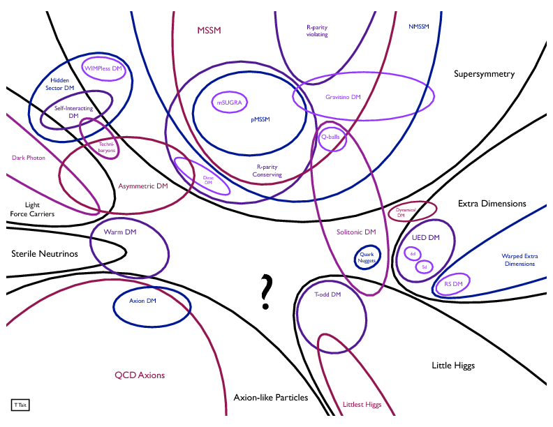